LqdSprdGaussianGasDisp Module Verification
This module is used for liquid substances that after outflow their evaporation should be calculated and dispersion of evaporated gas should be considered (to calculate explosive gas). For this purpose, liquid spread was considered as same pool liquid with same parameters, and for gas evaporation rate and dispersion, the gaussian formula has been used. Verification of this model has been done in some steps using existing solved examples or handy calculations (in excel) and comparing with results of the software.
The below codes can be downloaded from here in Jupyter Notebook format. The excel file that independent calculations has been done inside it, can be downloaded from here.
To validate the module calculations, by the below code the calculated evaporated mass results compared with Casal book example 2.9:
Verification:
#Verification by casal example 2.9
opr.wipe()

SiteTAg=1
opr.Sites.Site(SiteTAg, Temperature=20+273,Pressure=1.0132*10**5 ,XSiteBoundary=[0,100,100,0], YSiteBoundary=[0,0,100,100], g=9.81)


#Create Wind Object
windobj=opr.WindData.WindRose(tag=1)
windobj.WindClass="A"
windobj.WindDirection=90
windobj.WindSpeed=3
windobj.AlphaCOEF=1
windobj.isCalmn=False


#Define Material
subsObj=opr.Substance.DataBank.CasCalEx2_1(1)
subsObj.Specific_Heat_of_Vaporization=392.23*1000
subsObj.Vapour_Pressure=16130                      #Accoring Casal Example 2.9
subsObj.Molecular_Weight=86/1000                   #Accoring Casal Example 2.9
subsObj.Boiling_Point=273+68.7                     #According Casal Example 2.9
subsObj.Liquid_Partial_Pressure_in_Atmosphere=0    #According Casal Example 2.9
subsObj.Lower_Flammability_Limit=0.03
subsObj.Upper_Flammability_Limit=3

#Define Outflow Models
tag=1
opr.OutFlowModel.TankHole(tag, Hole_Diameter=0.05, Hole_Height_FromBot=0, delta_t=100, Cd=1)

opr.Safety.Dike(tag=1, Height=10, Area=3.1415*11**2)

#Define Plant Units
xc=0
yc=0
D=5
#OnGroundTag=1
Uni=opr.PlantUnits.ONGStorage(1,SiteTag=SiteTAg,DikeTag=1,
                              Horizontal_localPosition=xc,Vertical_localPosition=yc,
                              Pressure=1.5*10**5 ,Temperature=2,
                              Diameter=5,Height=10,
                              SubstanceTag=1,SubstanceVolumeRatio=0.85) #Define a StorageTank


Uni.isdamaged=True

#These steps will be done Automatically By the Program inside the Analysis Part
OutFlowObj=opr.OutFlowModel.ObjManager[1]     # Get OutFlow Object
UnitObj=opr.PlantUnits.ObjManager[1]          # Get Unit Object
Subs=opr.Substance.ObjManager[1]              # Get Substance Object
SiteObj=opr.Sites.ObjManager[1]               # Get Site Object
UnitObj.OutFlowModelObject=deepcopy(OutFlowObj)  #Assign OutFlow Model to Unit Object
UnitObj.OutFlowModelObject.UnitObject=UnitObj
UnitObj.OutFlowModelObject.Calculate(); #Calculate OutFlow Calculations to get


#Define Dispesion Spread Models and their connections to the materials and outflows
DispObject=opr.DispersionSpreadModels.LqdSprdGaussianGasDisp(tag=1,MatTags=[1], OutFlowModelTags=[1,2,3,4]) #Creat the Dispersion Object
UnitObj.DispersionSpreadModelObject=DispObject           #Assign Dispersion Object to the Unit Object
UnitObj.DispersionSpreadModelObject.UnitObject=UnitObj   #Assign the UnitObject to the Dispersion Model
UnitObj.DispersionSpreadModelname=DispObject.name

#Do Calculations
DispObject.Calculate();
poolArea=max(DispObject.LiquidRadious)**2*3.1415
V=Uni.V_subs
md=max(DispObject.LiquidVaporizationMassRate)
E=md/poolArea
h=V/poolArea

print('The substance Height in Dike=',h)
print('Evaporation of mass per area (E)=',E)
print('Evaporation of mass md=',md)
print('Results are compatible with Casal Example 2.9 that md=0.851')
The result of above code has been shown in the following:
The substance Height in Dike= 0.43906253585224136
Evaporation of mass per area (E)= 0.002244769333550875
Evaporation of mass md= 0.853285086223359
Results are compatible with Casal Example 2.9 that md=0.851
Verification Part2:
In the following code, cross and longitudinal concentration of gas at specifies locations are checked by independent calculations in Excel. (The code should be run after the prior code in the above):
#Plot cross section of the plume Concentration values and longitudinal Concentration values
x=[i/10 for i in range(-100,110)]
C=[DispObject.GasConcentration(4,X,0.5) for X in x]

plt.figure()
plt.plot(x,C,label='Code Results')
plt.ylabel('C')
plt.xlabel('y')
plt.title('Concentration at x=4 and z=0.5')

excelx=[-18,-17.5,-17,-16.5,-16,-15.5,-15,-14.5,-14,-13.5,-13,-12.5,-12,-11.5,-11,-10.5,-10,-9.5,-9,-8.5,-8,-7.5,-7,-6.5,-6,-5.5,-5,-4.5,-4,-3.5,-3,-2.5,-2,-1.5,-1,-0.5,0,0.5,1,1.5,2,2.5,3,3.5,4,4.5,5,5.5,6,6.5,7,7.5,8,8.5,9,9.5,10,10.5,11,11.5,12,12.5,13,13.5,14,14.5,15,15.5,16,16.5,17,17.5,18,18.5,19,19.5]
excelC=[2.75050362807037E-08,5.78984378520003E-08,1.193481540838E-07,2.40912204831127E-07,4.76207393888374E-07,9.21780893949689E-07,0.000001747243791382,3.24319861356762E-06,5.89505445753405E-06,1.04929193064724E-05,1.82893840944468E-05,3.12173521940422E-05,5.21779825972259E-05,0.000085402923762687,0.000136883918911059,0.000214845547446069,0.000330213269180967,0.00049700060795634,0.000732509995219599,0.00105721770152036,0.00149420275599164,0.00206799210319344,0.00280273769730309,0.00371972017028715,0.00483428578211008,0.00615245728422463,0.00766759436872633,0.00935758731811342,0.0111831173664259,0.013087482479099,0.0149983533024595,0.016831595361829,0.0184969967501868,0.0199054222426646,0.0209766341887419,0.0216468371878843,0.0218749632829608,0.0216468371878843,0.0209766341887419,0.0199054222426646,0.0184969967501868,0.016831595361829,0.0149983533024595,0.013087482479099,0.0111831173664259,0.00935758731811342,0.00766759436872633,0.00615245728422463,0.00483428578211008,0.00371972017028715,0.00280273769730309,0.00206799210319344,0.00149420275599164,0.00105721770152036,0.000732509995219599,0.00049700060795634,0.000330213269180967,0.000214845547446069,0.000136883918911059,0.000085402923762687,5.21779825972259E-05,3.12173521940422E-05,1.82893840944468E-05,1.04929193064724E-05,5.89505445753405E-06,3.24319861356762E-06,0.000001747243791382,9.21780893949689E-07,4.76207393888374E-07,2.40912204831127E-07,1.193481540838E-07,5.78984378520003E-08,2.75050362807037E-08,1.27953401015458E-08,5.8288876128192E-09,2.60024197941628E-09]
plt.plot(excelx,excelC,label='Excel Results')
plt.legend()

z=0.5
x=[i/100 for i in range(-100,170)]
C=[DispObject.GasConcentration(X,0,z) for X in x]


plt.figure()
plt.plot(x,C,label='Code Results')
plt.ylabel('C')
plt.xlabel('x')
plt.title('Concentration at y=0 and z=0.5')

excelx=[-1,-0.95,-0.9,-0.85,-0.8,-0.75,-0.7,-0.65,-0.6,-0.55,-0.5,-0.45,-0.4,-0.35,-0.3,-0.25,-0.2,-0.15,-0.0999999999999997,-0.0499999999999997,3.19189119579733E-16,0.0500000000000003,0.1,0.15,0.2,0.25,0.3,0.35,0.4,0.45,0.5,0.55,0.6,0.65,0.700000000000001,0.750000000000001,0.800000000000001,0.850000000000001,0.900000000000001,0.950000000000001,1,1.05,1.1,1.15,1.2,1.25,1.3,1.35,1.4,1.45,1.5,1.55,1.6,1.65,1.7,1.75,1.8,1.85,1.9,1.95,2,2.05,2.1,2.15,2.2,2.25,2.3,2.35,2.4,2.45,2.5,2.55,2.6,2.65,2.7,2.75]
excelC=[0,0,0,0,0,0,0,0,0,0,0,0,0,0,0,0,0,0,0,0,0,0.162423892233286,1.96268547574951,2.08831220306757,1.68587582341667,1.31309998590647,1.03310917766095,0.828613617339742,0.677733807163529,0.564234370189099,0.477076901346487,0.408835884324658,0.35445914467813,0.310446658467203,0.274326546239493,0.244320852205319,0.219129154922523,0.197785279752448,0.179560152695431,0.163894689817027,0.150352919493861,0.138589091386733,0.128324568560311,0.119331557667395,0.111421581353949,0.104437208531498,0.0982460081736155,0.0927360202223179,0.0878122702114609,0.0833940149263856,0.0794125140841289,0.0758091933134559,0.0725341086620575,0.0695446511868096,0.0668044479339553,0.0642824268059441,0.0619520200177139,0.0597904856694526,0.0577783303723033,0.0558988184257281,0.0541375550848942,0.0524821331548172,0.0509218336047612,0.0494473721664283,0.0480506849941132,0.0467247474438855,0.045463420886149,0.0442613232134041,0.0431137193534885,0.0420164286582596,0.0409657465184507,0.0399583779666248,0.0389913813804806,0.038062120696258,0.0371682247938889,0.0363075529283366]
plt.plot(excelx,excelC,label='Excel Results')
plt.legend()
The results of above code are shown in the following figures.
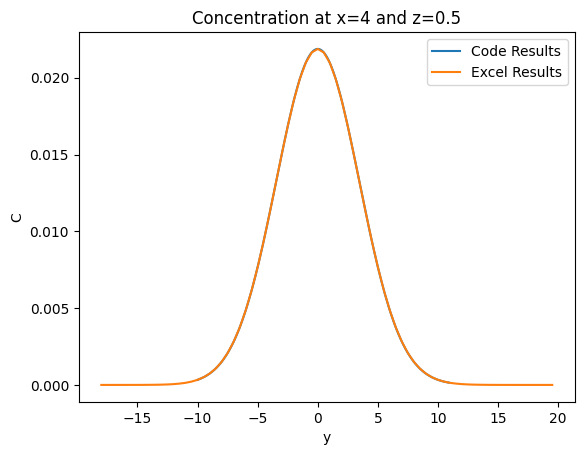
Calculated cross concentration of plume and compare results with independent calculations
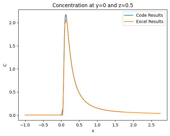
Calculated longitudina concentration of plume and compare results with independent calculations
Verification Part3:
In this part location of center line of plume is checked again by independent calculations in excel. (The code should be run after the prior code in the above):
#Another Example to show the centyer line and dispersed gas and ...
#Calculate center line

LFL=0.03
UFL=3

x,z,zt,yl,xpoints,ypoints,zpoints,Dx,Dy,Dz,Conc=DispObject._GasPoints(LFL,UFL,SegmentNumbers=10,errpercent=1)

plt.figure()
plt.plot(x,z,label='Code Centerline')
plt.ylabel('z')
plt.xlabel('x')

plt.title('Center Line of Concentration plume')

excelX=[0.01,0.5,0.7,1,1.04,1.05,1.45,1.9,2,3]
excelC=[0.439062536,0.439062536,0.439062536,0.429062536,0.429062536,0.429062536,0.319062536,0.009062536,0.009062536,0.009062536]
plt.plot(excelX,excelC,label='Excel Centerline')
plt.legend()
The results of above code are shown in the following figures.
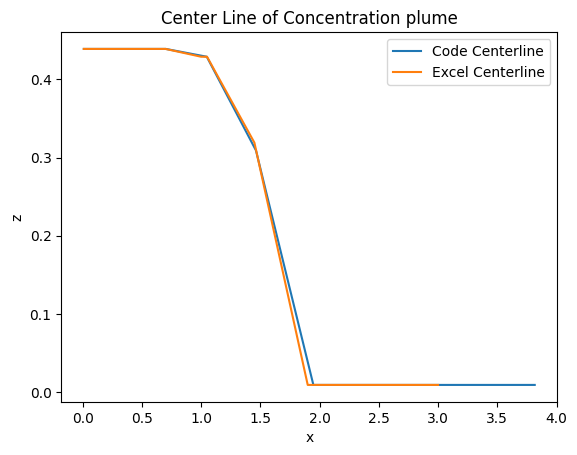
Center line of plume and compare results with independent calculation
Verification Part4:
Also, the module empowered to an algorithm to calculate the mass and its center of the dispersed gas. This algorithm uses the centerline values and for each center line, depend on its deviation in each cross direction, it selects number of points that covers the spaces that have concentration greater than LFL. By this way in a very short time the dispersed gas mass and its center will be calculated. To check the validation on the generated space and calculated mass and center, the following controls has been done using Excel.
By considering the number of the segments equal to 1000 (a very huge number and 10 is enough and has enough accuracy) the maximum distance from center of the release becomes equal to x=3.47 m . The example LFL is equal to LFL=0.03, so we expect that for any point greater than 3.5m we have no point greater than LFL. To check this condition for x=3.5 and on y=0 we check the all values on the z axis. The results are shown in the following figure. As it can be seen all values on x=3.5 are less than LFL limitation and the maximum point on the ground is equal to LFL that shows we have no volume to be consider in mass calculations.
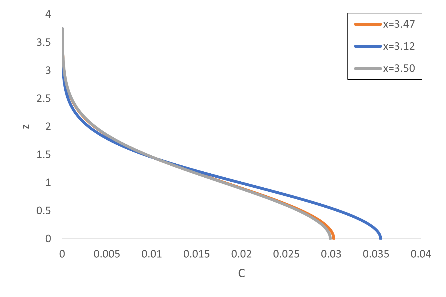
Variation of the Concentration along the height at different distances from source
For 1000 segments the calculated mass and center of the mass is equal to \(M=0.60 kg\) and Center of the mass is \((x=1.36,y=0,z=0.380)\) and for 10 segments it is equal to \(M=0.656 kg\) and center of the mass is \((x=1.33,y=0,z=0.382)\).
To get ensure that Center of mass and mass are calculated correctly, for calculated points, the concentration are calculated and then center of the mass and mass also are calculated separately using excel and the results checks with code for 10 segments. As it is shown in Table 1 results are fully compatible as expected.
Validation on Mass Calculations Formula
Module
Excel
\[Mass (\Sigma M_i)\]\[0.656\]\[0.656\]\[\Sigma M_i\times x_i\]\[-\]\[0.8737\]\[\Sigma M_i\times z_i\]\[-\]\[0.251\]\[X\]\[1.332\]\[Y\]\[0.382\]\[0.382\]Calculated point for 10, 50, 100 and 300 segments, also are shown in the following html figures:
Verification by: Bijan Sayyafzadeh